CALCULUS
Areas of Focus:
- Differentiation
- Maximization and minimization
- Partial derivatives
- Integration
- Integration over a line
- Double integrals
- Integration over an area
- Centroid of an area
- Integrating differential equations
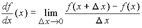
The derivative of a function is a measure of how the function changes as a
result of a change in the value of its argument. Given the function f(x),
the derivative of f with respect to x is written as  or
as
or
as  , and is defined by
As shown in the figure, the derivative of the function f(x) at point x gives the slope of the function at x in terms of the ratio of the rise divided by the run for the line AB that is tangent to the curve at point x.
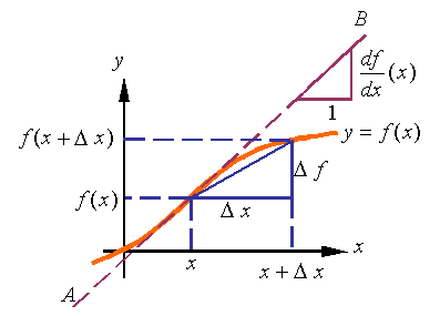
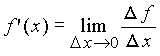
The derivative of the function f(x) is also sometimes written as f ' (x). As shown in the figure, one can also write the definition of the derivative as
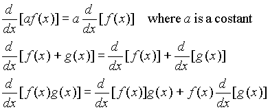
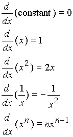
The basic rules of differentiation are
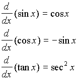
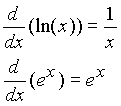
The derivative of commonly used functions:
The following is a list of the derivatives of some of the more commonly used functions.
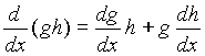
The product rule for derivatives:
Consider a function such as f(x)=g(x)h(x) that is the product of two functions. The product rule can be used to calculate the derivative of f with respect to x. The product rule states that
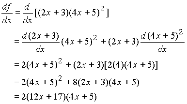
For example, To take the derivative of f(x)=(2x+3)(4x+5)2 one can follow these steps
The chain rule for derivatives:
Consider the function f(U), where U is a function of x. One can calculate the derivative of f with respect to x by using the chain rule given by
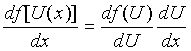
For example, to calculate the derivative of f(U) = Un with respect to x, where U = x2+a, one can follow these steps
Maximization
and minimization:
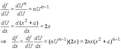
A point on a smooth function where the derivative is zero is a local maximum, a local minimum, or an inflection point of the function. This can be clearly seen in the figure, where the function has three points at which the tangent to the curve is horizontal (the slope is zero). This function has a local maximum at A, a local minimum at B, and an inflection point at C.
One can determine whether a point with zero derivative is a local maximum, a local minimum, or an inflection point by evaluating the value of the second derivative at that point.
Given a smooth function f(x), one can find the local maximums, local minimums, and inflections points by solving the equation

to get all points x that have a derivative of zero. One can then check the second derivative for each point to get the specific character of the function at each point.
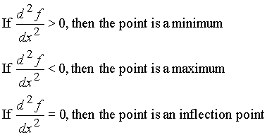
Global maximum and minimum:
The global maximum or minimum of a smooth function in a specific interval of its argument occurs either at the limits of the interval or at a point inside the interval where the function has a derivative of zero. As can be seen in the figure, the function shown has a global maximum at point A on the left boundary of the interval under consideration, a global minimum at B, a local maximum at C, and a local minimum at D.
The derivative of a function of several variable with respect to only one of
its variables is called a partial derivative. Given a function f(x,y),
its partial derivative with respect to its first argument is denoted by ![]() and
defined by
and
defined by
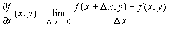
Since all other variables are kept constant during the partial derivative, it represents the slope of the curve one obtains when varying only the designated argument of the function.
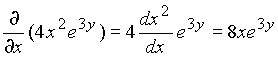
For example, the partial derivative of the function ![]() with respect to x
is evaluated by treating y as a constant so that one gets
with respect to x
is evaluated by treating y as a constant so that one gets
The chain rule:
Consider a function f[U(x), V(x)] of two arguments U and V, each a function of x. The chain rule can be used to find the derivative of f with respect to x by the rule
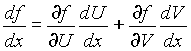
For example, consider the function f = UV2 where U =2x+3 and V=4x2. The derivative of f with respect to x is given by

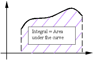
The integral of a function f(x) over an interval from x1 to x2 yields the area under the curve of the function over this same interval.
Let F denote the integral of f(x) over the interval from x1 to x2. This is written as
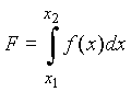
and is called a definite integral since the limits of integration are
prescribed. The area under the curve in the following figure can be approximated
by adding together the vertical strips of area ![]() . Therefore, the
integral is approximated by
. Therefore, the
integral is approximated by
![]()
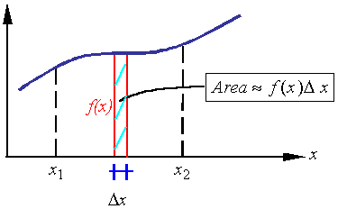
This approximation approaches the value of the integral as the width of the strips approaches zero.
Indefinite Integrals:
A function F(x) is the indefinite integral of the function f(x) if
The indefinite integral is also know as the anti-derivative. Since the derivative of a constant is zero, the indefinite integral of a function can only be evaluated up to the addition of a constant. Therefore, given a function F(x) to be an anti-derivative of f(x), the function F(x) + C, where C is any constant, is also an anti-derivative of f(x). This constant is known as the constant of integration and may be determined only if one has additional information about the integral. Normally, a known value of the integral at a specified point is used to calculate the constant of integration.
The basic rules of integration are
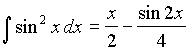
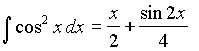
The indefinite integral of commonly used functions:
The following is a list of indefinite integrals of
commonly used functions, up to a constant of integration [![]() ]:
]:
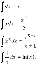
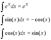
Note: Remember to add a constant of integration. You evaluate the constant of integration by selecting the constant of integration such that the integral passes through a known point.
Relating definite and indefinite integrals:
To obtain the value of the definite integral knowing the value of the indefinite integral of the function, one can subtract the value of the definite integral evaluated at the lower limit of integration from its value at the upper limit of integration. For example, if you have the indefinite integral
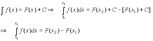
Note that C, the constant of integration, cancels in the subtraction and need not be included. It is common to sometimes use the notation
![]()
Change of variables:
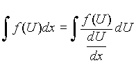
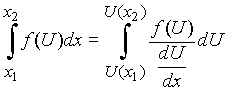
Given a function U(x), one can use 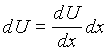 to
change the variable of integration from x to U . The change of
variables results in the rule
to
change the variable of integration from x to U . The change of
variables results in the rule
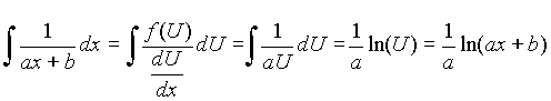
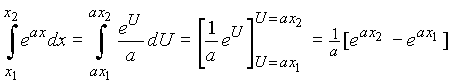
For example, given the function 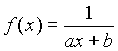 we can
write this function as
we can
write this function as ![]() where U = ax+b and
where U = ax+b and  . Therefore,
the integral of f can be evaluated by using the following steps.
. Therefore,
the integral of f can be evaluated by using the following steps.
Change of variables for a definite integral is similar with an additional change in the limits of integration. The resulting equation is
For example, given the function ![]() , we can
write this function as
, we can
write this function as ![]() where U = ax and . Therefore,
the integral of f can be evaluated by using the following steps.
where U = ax and . Therefore,
the integral of f can be evaluated by using the following steps.
Integration by parts:
Given the functions U(x) and V(x), one can use integration by parts to integrate the following integral using the relation
![]()
For example, to evaluate the integral
![]()
one can take ![]() and
and ![]() so that
so that ![]() and
and
![]() . Using integration by parts we get
. Using integration by parts we get
![]()
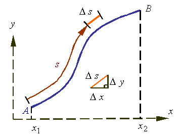
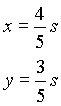
The integral F of function f(s) over line AB, that is defined by s = 0 to s = l, is written as
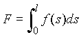 .
.
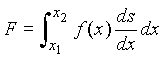
When either the domain of integration or the function is described in terms of another variable, such as x in the figure, one can evaluate F by a change of variables to get
Depending on the format the information is provided in, it might be necessary to use the Pythagorean Theorem to relate the differential line element along the arc of the curve to the x and y coordinates. For example, in the figure shown we can see that
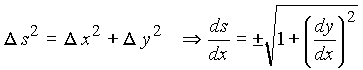
The sign of the root must be selected based on the specifics of the problem under consideration.
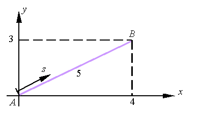
For example, consider integrating the function f(x,y) =xy2 over the straight line defined in the figure from point A to point B. Direct integration, using the relations
would yield
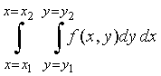
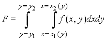
The double integral of function f(x,y) first integrating over x and then integrating over y is given by
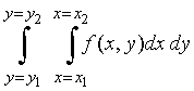
The notation implies that the inner integral over x is done first, treating y as a constant.
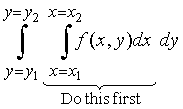
Once the inner integral is completed and the limits of integration for x are substituted into the expression, the outer integral is evaluated and the limits for y are substituted into the resulting expression. The rules of integration are the same as used for single integration for both the integration over x and the integration over y. To integrate over y first and then over x, the integration would be written as
One can also write the integral limits without specifying the variable (i.e., without using "x=" and "y="). The order dxdy or dydx clearly specifies what variable a specific limit is associated with.
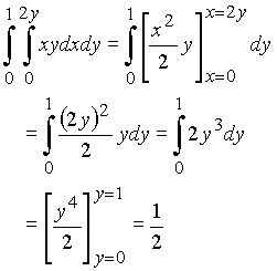
Consider the following example of double integration of the function f(x,y) =xy2.
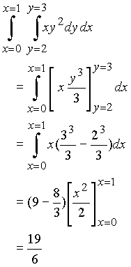
Unlike the example, the limits of integration need not be constants. There will be no problem as long as the inner integral is conducted fist and the limits are substituted into the resulting expression before the outer integral is evaluated. For example, consider the following integral.
The double integral F of the function ![]() over the area A
is written as
over the area A
is written as
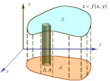
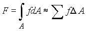
This integral is the sum of fdA over the area A. Each fdA
is the volume of the column with base dA and height f. Thus, the
integral gives the volume under the surface ![]() . To accomplish the summation
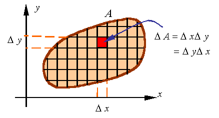
that is represented by the integral, one needs to section the domain of
integration A into small parts (i.e., into many small dAs). As shown in
the figure, the domain of integration can be sections into rectangular
sections, each with an area
. To accomplish the summation
that is represented by the integral, one needs to section the domain of
integration A into small parts (i.e., into many small dAs). As shown in
the figure, the domain of integration can be sections into rectangular
sections, each with an area ![]() . At the limit of small element sizes, the sum of
these area elements adds up to the original domain of integration.
. At the limit of small element sizes, the sum of
these area elements adds up to the original domain of integration.
The differential element of area dA in a rectangular x-y coordinate system is given by either dA=dxdy or dA=dydx. The difference between the two is the order of integration. If done correctly, the value of the integration does not depend on this selection, yet the ease of integration may strongly depend on the choice for dA. If dA=dxdy is selected, then for each value of y an integration over x is conducted from the left limit of the domain to its right limit. This process fills the domain with differential elements of area and is shown in the figure.
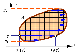
As can be seen from the figure, the limits of integration of x depend on the value of y so that the integral is written as
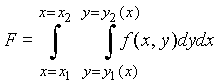
On the other hand, if one takes dA=dydx, the order of integration changes. In this case, for each x between x1 and x2, the argument is integrated over y from the lower limit of area to its upper limit. This is shown in the figure.
In this case the integral can be written as
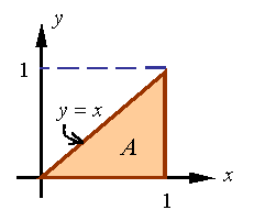
For example, consider the integral of f(x,y) =xy over the domain shown in the figure.
The integral can be defined as
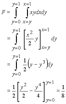
Alternately, one can get the integral from
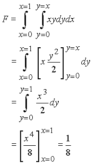
As can be seen, the result of the integration does not change based on the selection of the order of integration, yet the setup of the integrals does change.
Polar coordinates:
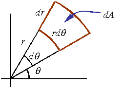
The differential element of area in polar coordinates is given by
![]()
This is a result of fact that the circumferential
sides of the differential element of area have a length of ![]() , as shown
in the figure. Otherwise the integration process is similar to rectangular
coordinates.
, as shown
in the figure. Otherwise the integration process is similar to rectangular
coordinates.
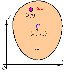
The centroid of an area is the area weighted average location of the given area. For example, consider a shape that is a composite of n individual segments, each segment having an area Ai and coordinates of its centroid as xi and yi. The coordinates of the centroid of this composite shape is given by
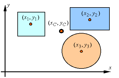
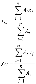
As can be seen, the location of each segment is weighted by the area of the segment and after addition divided by the total area of the shape. As such, the centroid represents the area weighted average location of the body. For a continuous shape the summations are replaced by integrations to get
where A is the total area.
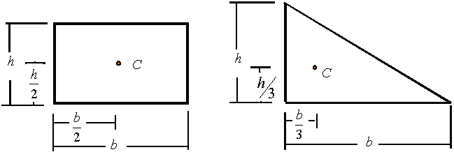
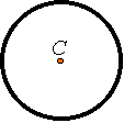
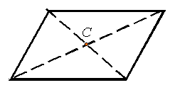
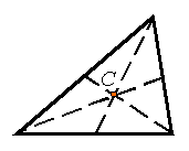
Centroid of common shapes:
The following figures show the centroid of some common objects, each indicated by a C.
Integration of
differential equations:
Differential equations are relations that are in terms of a function and its derivatives. There are some methods for solving these equations to find an explicit form of the function. Some of the simplest differential equations are of the form

The variables in such equations can be separated to get
![]()
and then integrated to get
![]()
where C is the constant of integration. A slightly more complicated differential equation is one of the form

The variables in such equations can be separated to get

and then integrated to get
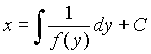
In general, if one can separate the variables, as was done in the two above examples, then one can use the methods of integration to integrate the differential equation.
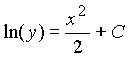
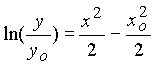
For example, consider the differential equation

The variables in this equation can be separated to give

The result of integrating this expression is
where the constant of integration can be found knowing a point (xo, yo) that the function must pass through. For this case
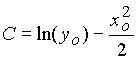
and the complete solution can be written as
If the variables cannot be separated directly, then other methods must be used to solve the equation.