An Introduction to Finite Element Methods
An Introduction to Finite Element Methods
Mehrdad Negahban
Department of Engineering Mechanics
University of Nebraska
Lincoln, NE 68588
1990-1991
Contents
1 A 1-D Example
1.1 Introduction
1.2 Steady State Heat Conduction in a Bar
1.2.1 Step 1: Formulation of the problem
1.2.2 Step 2: Formulation of the weak form
1.2.3 Step 3: Finite element approximation
1.2.4 Step 4: Assembling the stiffness matrix and load vector
1.3 An example
2 A 2-D Example
2.1 Step 1: The torsion problem
2.2 Step 2: The weak form of the torsion problem
2.3 Step 3: Discretization of the domain
2.4 Step 4: Finite element approximation of the weak form
3 Programing Considerations in FEM
3.1 Organization of finite element method programs
3.2 Elements, nodes, connectivity, etc.
3.3 Assembling the global stiffness matrix and load vector
3.4 Boundary conditions
3.5 Solving the system of equations
3.6 General comments
1.1 Introduction
The finite element method (FEM) is a numerical method to solve differential
equations. There are several basic steps to solving a problem by the FEM method.
These steps are:
- Formulation of the problem into a differential or integral equation.
- Development of the weak formulation of the problem.
- Finite element approximation of the domain and variables.
- Assembling the stiffness matrix and load vector and solving the problem.
- Post processing (analysis and presentation of the results).
1.2 Steady State Heat Conduction in a Bar
We will proceed to describe the steps in the finite element method by the aid
of an example. Consider the problem of heat conduction through a bar.
1.2.1 Step 1: Formulation of the problem
The problem under consideration is that of the steady state flow of heat
through a bar.
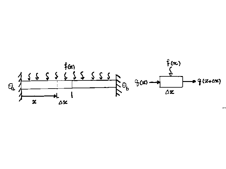
Figure 1.1: Steady state thermal conduction in a bar.
Figure 1.1 shows how heat flows through an element of this bar.
Balancing the heat entering and exiting this element gives
|
q(x) +f(x) \triangle x = q(x+\triangle x ) , |
| (1.1) |
where q is the heat flux along the bar and f(x) is the heat flow through the
lateral surfaces per unit length of the bar. Reorganizing
and taking the
limit as \triangle x goes to zero yields
Introducing Fourier's law of heat conduction ( q = - k[(d q)/dx])
into this equation results in
where q is the temperature and k is the coefficient of thermal
conduction.
Since the problem is a second order ordinary differential equation one can
prescribe two conditions. We will look at solving the above differential equation
subject to any one of the following boundary conditions:
- q = qa at x=a and q = qb at x=b ,
- q = qa at x=a and q=-k[(d q)/dx] = qb at x=b ,
- q=-k[(d q)/dx] = qa at x=a and q = qb at x=b , or
- q=-k[(d q)/dx] = qa at x=a and q=-k[(d q)/dx] = qb at x=b .
1.2.2 Step 2: Formulation of the weak form
The solution to this problem is a temperature field which satisfies the
differential equation
at every point in the bar. We will relax this requirement by replacing this
equation by
|
- |
ó
ő
|
Â
|
k |
q
|
|
d2 q
dx2
|
dx = |
ó
ő
|
Â
|
|
q
|
f(x) dx , |
| (1.5) |
where  is any region of the bar and [`(q)] is a test function. If
one requires that this equation hold for all possible test functions [`(q)],
it will be possible to get the original differential equation from this integral
equation. Any point in the bar can be isolated by selecting a test function
which is only positive and is nonzero only in a small region around that point.
The aim is not to require the integral equation to hold for all possible
[`(q)] functions, but to select a set of test functions and require the
integral equality to hold for this set of functions. Hence, we do not require
the differential equation to be exactly satisfied at all points, but require the
temperature field to only satisfy the integral equation for a select number
of test functions (we have weakened the original equation).
We will now use integration by parts to get the weak form of the problem as
|
-[k |
q
|
|
d q
dx
|
]x=ab + |
ó
ő
|
b
a
|
k |
dx
|
|
d q
dx
|
dx = |
ó
ő
|
b
a
|
|
q
|
f(x) dx , |
| (1.6) |
subject to the appropriate boundary conditions.
The application of integration by parts also introduces a weakening of the
problem since we are no longer required to have temperature fields which have a
second derivative. It is now only required that the temperature field have a
first derivative as can be seen from equation (1.6).
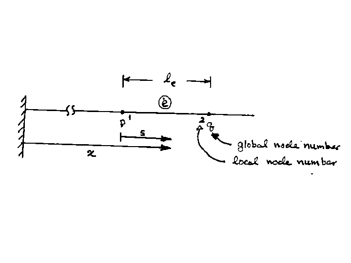
1.2.3 Step 3: Finite element approximation
We will use two node line elements to approximate both the temperature field and
the test functions. The length of the bar will be partitioned into ne elements
as shown in Figure 1.2. Each element has an element number and one node
at each end. Nodes are given two numbers. The global node number is one which is
unique for each node and which distinguishes it from all other nodes. For each
element there is also a local numbering system. For a two node element the local
nodes are distinguished in the element by designating a local node number of
1 to one node and 2 to the other node.
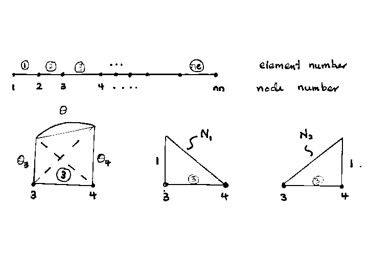 fig1-2.wmf fig1-2.wmf | |
|
Figure 1.2: Approximation of q and [`(q)] by the use of shape
functions.
The temperature and the test function will be approximated over
each element by
|
q = qe1N1(x)+qe2N2(x) = |
é
ë
|
|
ů
ű
|
|
é
ę
ë
|
|
ů
ú
ű
|
, |
| (1.7) |
and
|
|
q
|
= |
q
|
e
1
|
N1(x)+ |
q
|
e
2
|
N2(x) = |
é
ę
ë
|
|
ů
ú
ű
|
|
é
ę
ë
|
|
ů
ú
ű
|
, |
| (1.8) |
where qei is the value of q at local node i,
[`(q)]ei is
the value of [`(q)] at local node i, and Ni(x) are known functions of
x. The Ni are known as shape functions. The shape functions are
selected such that N1=1 at local node 1, N1=0 at local node 2, N2=0 at
local node 1, N2=1 at local node 2. For a two node line element
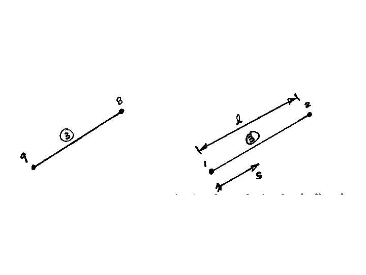
of length le and local coordinate s as shown in Figure 1.3, the shape
functions will be
and
The shape functions are selected such that the sum of the shape functions at
each point will add up to unity. It must be noted that the shape functions are
different for different elements, even though this is not made explicit in the
notation.
Figure 1.3: Relation between local and global coordinates.
The two integrals in the weak formulation of the problem, given in equation
(1.6), can each be written as a sum of integrals,
each integral being over one element. This can be written as
|
|
ó
ő
|
b
a
|
k |
dx
|
|
d q
dx
|
dx = |
ne
ĺ
e=1
|
|
ó
ő
|
We
|
k |
dx
|
|
d q
dx
|
dx, |
| (1.11) |
and
|
|
ó
ő
|
b
a
|
|
q
|
f(x) dx = |
ne
ĺ
e=1
|
|
ó
ő
|
We
|
|
q
|
f(x) dx , |
| (1.12) |
where We is the domain of element number e.
Over each element one can use the above approximations for the temperature and
test function to get
|
|
ó
ő
|
We
|
k |
dx
|
|
d q
dx
|
dx = |
ó
ő
|
le
0
|
k |
ds
|
|
d[qe1 N1 +q2 N2]
ds
|
ds , |
| (1.13) |
and
|
|
ó
ő
|
We
|
|
q
|
f(x) dx = |
ó
ő
|
le
0
|
[ |
q
|
e
1
|
N1 + |
q
|
e
2
|
N2] f(x) ds , |
| (1.14) |
since x=x1+s, where x1 is the location of the first node in the element.
Since qe1, qe2, [`(q)]e1, and [`(q)]e2 are constants,
one can write
|
|
dx
|
= |
ds
|
= |
é
ę
ë
|
|
ů
ú
ű
|
|
é
ę
ę
ę
ę
ę
ę
ę
ę
ę
ę
ë
|
|
ů
ú
ú
ú
ú
ú
ú
ú
ú
ú
ú
ű
|
, |
| (1.15) |
and
|
|
d q
dx
|
= |
d[qe1 N1 +qe2 N2]
ds
|
= |
é
ę
ę
ę
ë
|
|
ů
ú
ú
ú
ű
|
|
é
ę
ë
|
|
ů
ú
ű
|
. |
| (1.16) |
Substitution of these relations into the integrals of equations (1.13)
and (1.14) gives
|
|
ó
ő
|
We
|
k |
dx
|
|
d q
dx
|
dx = k |
é
ę
ë
|
|
ů
ú
ű
|
|
ó
ő
|
le
0
|
|
é
ę
ę
ę
ę
ę
ę
ę
ę
ę
ę
ë
|
|
ů
ú
ú
ú
ú
ú
ú
ú
ú
ú
ú
ű
|
|
é
ę
ę
ę
ë
|
|
ů
ú
ú
ú
ű
|
ds |
é
ę
ë
|
|
ů
ú
ű
|
, |
| (1.17) |
and
|
|
ó
ő
|
We
|
|
q
|
f(x) dx = |
é
ę
ë
|
|
ů
ú
ű
|
|
ó
ő
|
le
0
|
|
é
ę
ë
|
|
ů
ú
ű
|
f(x) ds . |
| (1.18) |
These equations can be written as
|
|
ó
ő
|
We
|
k |
dx
|
|
d q
dx
|
dx = [ |
q
|
e
|
]T [Ke][qe], |
| (1.19) |
and
|
|
ó
ő
|
We
|
|
q
|
f(x) dx = [ |
q
|
e
|
]T [fe] , |
| (1.20) |
where
|
[ |
q
|
e
|
] = |
é
ę
ę
ę
ę
ë
|
|
ů
ú
ú
ú
ú
ű
|
, |
| (1.21) |
|
[Ke] = |
é
ę
ë
|
|
ů
ú
ű
|
= k |
ó
ő
|
le
0
|
|
é
ę
ę
ę
ę
ę
ę
ę
ę
ë
|
|
ů
ú
ú
ú
ú
ú
ú
ú
ú
ű
|
ds, |
| (1.23) |
|
[fe] = |
é
ę
ë
|
|
ů
ú
ű
|
= |
ó
ő
|
le
0
|
|
é
ę
ë
|
|
ů
ú
ű
|
f(x) ds . |
| (1.24) |
The matrix [Ke] is known as the element stiffness matrix and the
matrix [fe] is known as the element load vector. For the shape
functions in (1.9) and (1.10) we have [(dN1)/ds] = -[1/(le)] and [(dN2)/ds] = [1/(le)]. Therefore, the element stiffness matrix can be written as
|
[Ke] = k |
ó
ő
|
le
0
|
|
é
ę
ę
ę
ę
ę
ę
ę
ę
ë
|
|
ů
ú
ú
ú
ú
ú
ú
ú
ú
ű
|
ds = |
é
ę
ę
ę
ę
ę
ę
ę
ę
ë
|
|
ů
ú
ú
ú
ú
ú
ú
ú
ú
ű
|
. |
| (1.25) |
To evaluate the element load vector one needs to know f(x). We will later calculate
this for a particular example.
The weak form of the problem can now be written as
|
[ |
q
|
q]x=ab + |
ne
ĺ
e=1
|
[ |
q
|
e
|
]T[Ke][qe] = |
ne
ĺ
e=1
|
[ |
q
|
e
|
]T[fe], |
| (1.26) |
where Fourier's law is used to replace the derivative of temperature in the
first term.
1.2.4 Step 4: Assembling the stiffness matrix and load vector
The next step is to organize the problem in the form of a set of algebraic
equations. Consider the example of a problem with two elements and three nodes
as shown in Figure 1.4. The two summations in equation (1.26)
can be written as
|
|
2
ĺ
e=1
|
[ |
q
|
e
|
]T[Ke][ |
q
|
e
|
] = |
é
ę
ë
|
|
ů
ú
ű
|
|
é
ę
ë
|
|
ů
ú
ű
|
|
é
ę
ë
|
|
ů
ú
ű
|
+ |
é
ę
ë
|
|
ů
ú
ű
|
|
é
ę
ë
|
|
ů
ú
ű
|
|
é
ę
ë
|
|
ů
ú
ű
|
|
|
|
= |
é
ę
ë
|
|
ů
ú
ű
|
|
é
ę
ę
ę
ë
|
|
ů
ú
ú
ú
ű
|
|
é
ę
ę
ę
ë
|
|
ů
ú
ú
ú
ű
|
, |
| (1.27) |
and
|
|
2
ĺ
e=1
|
[ |
q
|
e
|
][fe] = |
é
ę
ë
|
|
ů
ú
ű
|
|
é
ę
ë
|
|
ů
ú
ű
|
+ |
é
ę
ë
|
|
ů
ú
ű
|
|
é
ę
ë
|
|
ů
ú
ű
|
|
|
|
= |
é
ę
ë
|
|
ů
ú
ű
|
|
é
ę
ę
ę
ë
|
|
ů
ú
ú
ú
ű
|
|
| (1.28) |
Therefore, for this problem the weak formulation given in equation (1.29) can be put in the form
|
[ |
q
|
3
|
q3- |
q
|
1
|
q1] +[ |
q
|
]T [K][q] = [ |
q
|
][f], |
| (1.29) |
where [K] is known as the global stiffness matrix, [f] is known as the
global load vector, and
|
[ |
q
|
] = |
é
ę
ę
ę
ę
ę
ę
ę
ę
ë
|
|
ů
ú
ú
ú
ú
ú
ú
ú
ú
ű
|
, |
| (1.30) |
|
[K] = |
é
ę
ę
ę
ë
|
|
ů
ú
ú
ú
ű
|
= |
é
ę
ę
ę
ë
|
|
ů
ú
ú
ú
ű
|
, |
| (1.32) |
|
[f] = |
é
ę
ę
ę
ë
|
|
ů
ú
ú
ú
ű
|
= |
é
ę
ę
ę
ë
|
|
ů
ú
ú
ú
ű
|
. |
| (1.33) |
To illustrate the way in which one arrives at the final set of equations we will
write the expanded form of equation (1.29) in the form
|
[ |
q
|
3
|
q3- |
q
|
1
|
q1] + |
é
ę
ë
|
|
ů
ú
ű
|
|
é
ę
ę
ę
ë
|
|
ů
ú
ú
ú
ű
|
|
é
ę
ę
ę
ë
|
|
ů
ú
ú
ú
ű
|
= |
é
ę
ë
|
|
ů
ú
ű
|
|
é
ę
ę
ę
ë
|
|
ů
ú
ú
ú
ű
|
. |
| (1.34) |
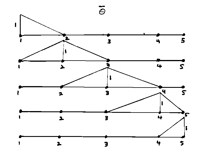
The test functions [`(q)] are arbitrary functions which we will select in
the manner shown in Figure 1.4. Three test functions are selected since
we will have three unknowns in this problem ( q1, q2,
q3; q1, q2, q3; q1, q2, q2; or
q1, q2, q2). Each test function provides one algebraic equation
for the unknowns. As can be seen from Figure 1.4, the first test
function has [`(q)]1 = 1, [`(q)]2 = 0, and [`(q)]3 = 0. The
second test function has [`(q)]1 = 0, [`(q)]2 = 1, and [`(q)]3 = 0. The third test function has [`(q)]1 = 0, [`(q)]2 = 0, and
[`(q)]3 = 1.
Figure 1.4: Test functions used to get the final form of the equation.
The following three equations are obtained from the substitution of the
selected test functions into equation (1.34).
|
-q1 + K11q1 +K12 q2 +K13q3 = f1 , |
|
|
K21q1 +K22 q2 +K23q3 = f2 , |
|
|
q3+K31q1 +K32 q2 +K33q3 = f3 . |
| (1.35) |
These equations can now be solved for the three unknowns.
If q1 and q3 are specified, then this system can be written as
|
|
é
ę
ę
ę
ë
|
|
ů
ú
ú
ú
ű
|
|
é
ę
ę
ę
ë
|
|
ů
ú
ú
ú
ű
|
= |
é
ę
ę
ę
ë
|
|
ů
ú
ú
ú
ű
|
. |
| (1.36) |
This would be the problem which one would solve if this was a well posed
problem. It turns out that this particular set of boundary values are not
proper.
Since the temperature is not fixed at any point in the bar, the temperature
profile can slide up and down. An examination of the stiffness matrix shows that
its determinant is zero (i.e., the system is singular).
If q1 and q3 are specified, then the middle equation can be used
to find q2, and the first and last equation are used to find the heat
flux at the two ends. The, mixed type boundary conditions can also be solved in
a similar manner.
Before we proceed it is important to state that in practice the boundary
conditions are not imposed as was presented above.
Theoretically, if we have known values of temperature at the boundary we
should eliminated these known values from the set of unknowns and introduce
the
unknown heat fluxes in the boundary term into the list of unknowns.
To avoid this complex procedure, the penalty method is used for
imposing the temperature boundary. This method modifies the stiffness
matrix and load vector to fix the value of temperature to a given value at
a boundary node.
The method is based on the fact that for any boundary node i there will be an
equation
|
Kii qi + other terms = fi . |
| (1.37) |
To impose the condition qi = [^(q)] one can add a term
pKiiqi to the left hand side of the equation and the term pKii[^(q)] to the right hand side of the equation to get
|
Kii qi + pKiiqi + other terms = fi+pKii |
^
q
|
|
| (1.38) |
where p is a large number. After dividing by pKii one gets
|
|
qi
p
|
+ qi+ |
other terms
pKii
|
= |
fi
pKii
|
+ |
^
q
|
|
| (1.39) |
All
term in this equation become small accept the two newly added ones.
Therefore, the equation will
become dominated by the equation qi = [^(q)] and the other terms
become unimportant. Since the method eliminates the importance of any other
terms entering this equation, it will not be necessary to introduce the unknown
heat flux into the list of unknowns.
In short, to impose a temperature boundary condition at global node i one can
multiply Kii in the stiffness matrix by (1+p) (i.e., add pKii to
Kii), and add pKii[^(q)] to fi. To impose a heat flux boundary
condition at global node j one adds q to fj, where
q is a heat flux directed into the bar.
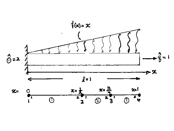
1.3 An example
As an example consider the problem of the bar shown in Figure 1.5. The
bar is of length l=1, is connected to a constant temperature thermal bath of
temperature [^(q)]=2 from the left and heat is being drawn from it at a
constant rate [^q]=1 from the right. The heat flow into the bar per unit
length from the lateral surfaces is given by f(x)=x. The coefficient of
thermal conduction k = 1.
Figure 1.5: Example problem.
Three two node line elements are selected as shown in Figure 1.5. The local stiffness matrices
can be calculated using equation (1.25) and will be
The global stiffness matrix will, therefore, be
The load vectors can be calculated using equation (1.24). Using equation
(1.9) and (1.10), the shape
functions for the first element are
Therefore,
|
f11 = |
ó
ő
|
[1/2]
0
|
(1-2x)x dx = |
1
24
|
, |
|
|
f12 = |
ó
ő
|
[1/2]
0
|
2x2 dx = |
1
12
|
. |
|
The shape functions for the second element are
|
N1 = 1-4(x- |
1
2
|
), N2 = 4(x- |
1
2
|
). |
|
Therefore,
|
f21 = |
ó
ő
|
[3/4]
[1/2]
|
[1-4(x- |
1
2
|
) ]x dx = |
7
96
|
, |
|
|
f22 = |
ó
ő
|
[3/4]
[1/2]
|
4(x- |
1
2
|
) x dx = |
1
12
|
. |
|
The shape functions for the third element are
|
N1 = 1-4(x- |
3
4
|
), N2 = 4(x- |
3
4
|
). |
|
Therefore,
|
f31 = |
ó
ő
|
1
[3/4]
|
[1-4(x- |
3
4
|
) ]x dx = |
5
48
|
, |
|
|
f32 = |
ó
ő
|
1
[3/4]
|
4(x- |
3
4
|
) x dx = |
11
96
|
. |
|
The global load vector will become
|
[f] = |
é
ę
ę
ę
ę
ę
ę
ę
ę
ę
ę
ę
ę
ę
ę
ę
ę
ę
ę
ę
ę
ę
ë
|
|
ů
ú
ú
ú
ú
ú
ú
ú
ú
ú
ú
ú
ú
ú
ú
ú
ú
ú
ú
ú
ú
ú
ű
|
. |
|
The problem that we must solve is
|
|
é
ę
ę
ę
ę
ë
|
|
ů
ú
ú
ú
ú
ű
|
|
é
ę
ę
ę
ę
ë
|
|
ů
ú
ú
ú
ú
ű
|
= |
é
ę
ę
ę
ę
ę
ę
ę
ę
ę
ę
ę
ę
ę
ę
ę
ę
ę
ę
ę
ę
ę
ë
|
|
ů
ú
ú
ú
ú
ú
ú
ú
ú
ú
ú
ú
ú
ú
ú
ú
ú
ú
ú
ú
ú
ú
ű
|
, |
|
where p is a large number and the stiffness matrix and load vectors have been
modified to impose the boundary
conditions.
For p=1 the solution will be
|
|
é
ę
ę
ę
ę
ë
|
|
ů
ú
ú
ú
ú
ű
|
= |
é
ę
ę
ę
ę
ę
ę
ę
ę
ę
ę
ę
ę
ę
ę
ę
ę
ę
ę
ę
ę
ę
ë
|
|
ů
ú
ú
ú
ú
ú
ú
ú
ú
ú
ú
ú
ú
ú
ú
ú
ú
ú
ú
ú
ú
ú
ű
|
= |
é
ę
ę
ę
ę
ë
|
|
ů
ú
ú
ú
ú
ű
|
. |
|
For p=10 the solution is
|
|
é
ę
ę
ę
ę
ë
|
|
ů
ú
ú
ú
ú
ű
|
= |
é
ę
ę
ę
ę
ę
ę
ę
ę
ę
ę
ę
ę
ę
ę
ę
ę
ę
ę
ę
ę
ę
ë
|
|
ů
ú
ú
ú
ú
ú
ú
ú
ú
ú
ú
ú
ú
ú
ú
ú
ú
ú
ú
ú
ú
ú
ű
|
= |
é
ę
ę
ę
ę
ë
|
|
ů
ú
ú
ú
ú
ű
|
. |
|
For p=100 the solution is
|
|
é
ę
ę
ę
ę
ë
|
|
ů
ú
ú
ú
ú
ű
|
= |
é
ę
ę
ę
ę
ę
ę
ę
ę
ę
ę
ę
ę
ę
ę
ę
ę
ę
ę
ę
ę
ę
ë
|
|
ů
ú
ú
ú
ú
ú
ú
ú
ú
ú
ú
ú
ú
ú
ú
ú
ú
ú
ú
ú
ú
ú
ű
|
= |
é
ę
ę
ę
ę
ë
|
|
ů
ú
ú
ú
ú
ű
|
. |
|
The exact solution is
which yields
|
|
é
ę
ę
ę
ę
ë
|
|
ů
ú
ú
ú
ú
ű
|
= |
é
ę
ę
ę
ę
ę
ę
ę
ę
ę
ę
ę
ę
ę
ę
ę
ę
ë
|
|
ů
ú
ú
ú
ú
ú
ú
ú
ú
ú
ú
ú
ú
ú
ú
ú
ú
ű
|
= |
é
ę
ę
ę
ę
ë
|
|
ů
ú
ú
ú
ú
ű
|
. |
|
Comparison of the exact solution and the finite element method solution shows
that for p=100 there is less than 1% error in the finite element solution.
The following is an example of how to solve a two dimensional problem using the
finite element method. The problem under consideration is the torsion of a
noncircular member.
2.1 Step 1: The torsion problem
The differential equation for the torsion problem is given by
|
|
¶2 f
¶x2
|
+ |
¶2 f
¶y2
|
= -2Gq, |
| (2.1) |
where f is a function of x and y and is called the potential
function, G is the shear modulus, and q
is the amount of twist per unit length of the bar.1
To solve the torsion problem
one must solve for the potential function f which satisfies this
differential equation at every point in the cross section W
and which also satisfies the boundary conditions
on the boundary curve ¶W.
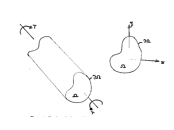
Figure 2.1: Torsion of a bar with an arbitrary cross section.
If one defines the gradient operator in the x-y plain as
then one will have
Therefore, one can write the problem as
and
In this problem the shear stress at any point of the cross section can be found
from f using
|
txy = |
¶f
¶z
|
and txz = - |
¶f
¶y
|
. |
| (2.7) |
The torque T required to crate a twist of q is given by
where dA is the differential element of area.
2.2 Step 2: The weak form of the torsion problem
In a simple way one can describe the generation of the weak form of an equation
as follows.
If for every c one can show ca = cb, then one can conclude that a=b. The
weak form of equation a=b in this case is ca=cb.
To formulate the weak form of the torsion problem we will multiply both sides of
(2.5) by a arbitrary potential function [`(f)](x,y). This will
give the relation
Since this equation must hold for every point in the cross section W, we
can integrate this relation over any region  of the cross section to get
|
|
ó
ő
|
Â
|
|
f
|
Ń°ŃfdA = -2 |
ó
ő
|
Â
|
G q |
f
|
dA . |
| (2.10) |
This equation is regarded as the weak form of the differential equation
(2.5). For this equation to be equal to equation (2.5), this
relation must hold for every function [`(f)].
We will rewrite equation (2.10) in a more convenient form using first the
relation
|
Ń°( |
f
|
Ńf) = |
f
|
Ń°Ńf+Ń |
f
|
°Ńf. |
| (2.11) |
Substitution of [`(f)] Ń°Ńf from this equation into
(2.10) yields
|
|
ó
ő
|
Â
|
Ń°( |
f
|
Ńf) dA - |
ó
ő
|
Â
|
Ń |
f
|
°ŃfdA = -2 |
ó
ő
|
Â
|
G q |
f
|
dA . |
| (2.12) |
Next we use the divergence theorem which states
|
|
ó
ő
|
Â
|
Ń°v dA = |
ó
ő
|
C
|
v °n ds , |
| (2.13) |
for every vector v and where n is the outward normal to C and
ds is the differential element of length along C.
Selecting v = [`(f)]Ńf one can convert the first integral
over  into an integral over C. This results into the final weak
form of the equation as
|
|
ó
ő
|
C
|
|
f
|
Ńf°n dA - |
ó
ő
|
Â
|
Ń |
f
|
°ŃfdA = -2 |
ó
ő
|
Â
|
G q |
f
|
dA . |
| (2.14) |
2.3 Step 3: Discretization of the domain
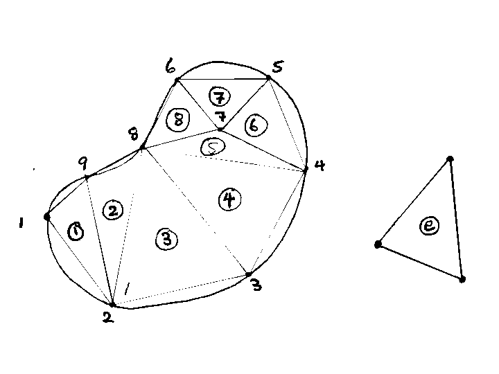
The third step is to discretize the domain. Here we will use the three node
triangular element which is the simplest two dimensional element to discretize
the cross section W. Figure
2.2 shows this element. This three node triangular element has one
node at each of its corners.
Figure 2.2: Three node triangular elements used to discretize the cross section
W.
Figure 2.2 also shows an example of how the
domain of the cross section can be modeled using this element.
In this example the domain is modeled by six triangular elements. The
element number is denoted by a number contained in a circle. This model of the
domain is called
a finite element mesh. This particular mesh has seven nodes.
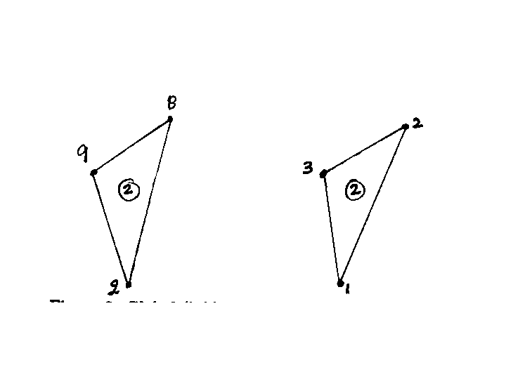
The nodes in each element have both a ``local node number'' and a ``global node
number''. The global node number refers to the node numbers given when
discretize the domain. Each element also has a set of local node numbers.
In this case the local node numbers for each element are 1, 2, and 3. For
example, Figure 2.3 shows both the local and global node numbers for
element 2. As can be seen from the figure the local node 1 refers to the global
node 2, the local node 2 refers to the global node 8 and the local node 3 refers
to the global node 9.
Figure 2.3: Global (left) and local (right) node numbers for element 2.
There is no order in how one numbers the elements and gives the global node
numbers. To avoid keeping track of sign changes, in this problem we will always
select local node numbers as counter-clock-wise.
It is essential that we have a method for going from the local node numbers
to the global node number. To do this we will introduce node connectivity which is
a matrix denoted by IJK(I,N), where IJK is the global node number for a node
with a local node number I in element N. As an example consider the local and
global node numbers given in Figure 2.3. The connectivity for element 2
will be given by
|
IJK(1,2)=2 , IJK(2,2)=8 , IJK(3,2)=9 . |
| (2.15) |
The function f is approximated on each element by
|
f = f1 N1(x,y) +f2 N2(x,y) +f3 N3(x,y) , |
| (2.16) |
where f1, f2, and f3 are the values of f at local node
number 1, 2, and 3, respectively, and N1, N2 and N3 are known functions
of x and y. Ni are known as shape functions. Let (x1,y1), (x2,y2) and (x3,y3) denote the coordinates of the three nodes of an element.
The three conditions f(x1,y1) = f1, f(x2,y2) = f2 and
f(x3,y3) = f3 can be satisfied by nine restrictions on the three
Ni. At the first node
|
N1(x1,y1) = 1, N2(x1,y1) = 0, N3(x1,y1)=0 . |
| (2.17) |
At the second node
|
N1(x2,y2) = 0, N2(x2,y2) = 1, N3(x2,y2)=0 . |
| (2.18) |
At the third node
|
N1(x3,y3) = 0, N2(x3,y3) = 0, N3(x3,y3)=1 . |
| (2.19) |
Since there are three restrictions on each shape function, one can represent
each shape function by a linear function of x an y and solve for the unknown
constants. Let us select for each element e the shape functions
where the value of the constants for each element can be evaluated from the above
restrictions on Ni. To simplify the notation, we will leave out the
superscript e from the notation.
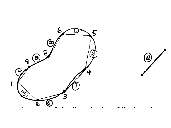
Since in addition to the area integrals we have line integrals on the boundary,
we need to discretize the boundary ¶W. For the boundary we
will use two node line elements. In this case each element has one node at each
end. Figure 2.4 shows the discretization of the boundary. As in the
discretization of the area, we have both a local and a global numbering system for
the nodes. The connectivity of these two numbering systems is given by a matrix
IJ(I,N), where IJ is the global node number for local node I of element N.
Figure 2.4: Line elements and the discretization of the boundary
The function f in the boundary will be approximated by a function of the
form
|
f = f1 |
^
N
|
1
|
(x,y) +f2 |
^
N
|
2
|
(x,y) , |
| (2.23) |
where f1 and f2 are the values of f at the two nodes and
[^N]1 and [^N]2 are the shape functions. Using a local coordinate
system as shown in figure 2.5, one can write these shape functions as
|
|
^
N
|
1
|
= 1- |
s
l
|
, and |
^
N
|
2
|
= |
s
l
|
|
| (2.24) |
Figure 2.5: Local coordinate s and local node numbering for the line element.
It must be mentioned that the sum of the shape functions at each point of the
element must equal unity. This can be used as a check to see if one has
selected the right shape functions.
2.4 Step 4: Finite element approximation of the weak form
For a problem with NN number of nodes the goal is to set the problem in the form
where [K] is an (NN,NN) matrix of constants known as the global stiffness
matrix, { f} is the (NN,1) matrix of unknown values of f at the nodes, and
{ f} is known as the global load vector and is an (NN,1) matrix of known constants.
Once the problem is set into this form one can use a linear equation solver to
get the unknown f.
Selecting the region  in equation (2.14) as the region of one
element We, one can get one equation for each element. Adding these
equations over all the elements one gets
|
|
NBE
ĺ
e=1
|
|
ó
ő
|
¶We
|
|
f
|
Ńf°nds - |
NE
ĺ
e=1
|
|
ó
ő
|
We
|
Ń |
f
|
°ŃfdA = -2 |
NE
ĺ
e=1
|
|
ó
ő
|
We
|
Gq |
f
|
dA , |
| (2.26) |
where NE is the number of elements and NBE is the number of boundary elements.
Note that the boundary integrals on the internal boundary between any two
adjacent elements cancels out of the summation leaving only the boundary
integral over ¶W.
On each element we will use the approximations for f and [`(f)] as
|
f = f1 N1 + f2 N2 + f3 N3 , |
| (2.27) | |
f
|
= |
f
|
1
|
N1 + |
f
|
2
|
N2 + |
f
|
3
|
N3 , |
| (2.28) |
|
where it is understood that the numbers refer to local node numbers for element
e, and that the Ni are the shape functions for element e.
This equation can be written as
and
|
|
f
|
= |
é
ę
ë
|
|
|
ů
ú
ű
|
|
é
ę
ę
ę
ë
|
|
|
ů
ú
ú
ú
ű
|
|
| (2.30) |
The derivatives of f and [`(f)] can be written as
|
|
¶f
¶x
|
= |
é
ę
ę
ę
ë
|
|
|
ů
ú
ú
ú
ű
|
|
é
ę
ę
ę
ë
|
|
|
ů
ú
ú
ú
ű
|
, |
| (2.31) |
|
|
¶f
¶y
|
= |
é
ę
ę
ę
ë
|
|
|
ů
ú
ú
ú
ű
|
|
é
ę
ę
ę
ë
|
|
|
ů
ú
ú
ú
ű
|
, |
| (2.32) |
|
|
¶x
|
= |
é
ę
ë
|
|
|
ů
ú
ű
|
|
é
ę
ę
ę
ę
ę
ę
ę
ę
ę
ę
ę
ę
ę
ę
ë
|
|
|
ů
ú
ú
ú
ú
ú
ú
ú
ú
ú
ú
ú
ú
ú
ú
ű
|
, |
| (2.33) |
|
|
¶y
|
= |
é
ę
ë
|
|
|
ů
ú
ű
|
|
é
ę
ę
ę
ę
ę
ę
ę
ę
ę
ę
ę
ę
ę
ę
ë
|
|
|
ů
ú
ú
ú
ú
ú
ú
ú
ú
ú
ú
ú
ú
ú
ú
ű
|
. |
| (2.34) |
The first equation for the area integral over We can be written as
|
|
ó
ő
|
We
|
Ń |
f
|
°ŃfdA = |
ó
ő
|
We
|
|
¶x
|
|
¶f
¶x
|
+ |
¶y
|
|
¶f
¶y
|
dA . |
| (2.35) |
The first term of this equation can be written as
|
|
ó
ő
|
We
|
|
¶x
|
|
¶f
¶x
|
dA = |
é
ę
ë
|
|
|
ů
ú
ű
|
|
ó
ő
|
We
|
|
é
ę
ę
ę
ę
ę
ę
ę
ę
ę
ę
ę
ę
ę
ę
ë
|
|
|
ů
ú
ú
ú
ú
ú
ú
ú
ú
ú
ú
ú
ú
ú
ú
ű
|
|
é
ę
ę
ę
ë
|
|
|
ů
ú
ú
ú
ű
|
dA |
é
ę
ę
ę
ë
|
|
|
ů
ú
ú
ú
ű
|
. |
| (2.36) |
A similar expression can be obtained for the second term of this integral.
Therefore, this integral can be represented as
|
|
ó
ő
|
We
|
Ń |
f
|
°ŃfdA = [ |
f
|
]T[Ke][f] , |
| (2.37) |
where [Ke] is the element stiffness matrix given by
|
[Ke] = |
ó
ő
|
We
|
|
é
ę
ę
ę
ę
ę
ę
ę
ę
ę
ę
ę
ę
ę
ę
ë
|
|
| |
|
¶N1
¶x
|
|
¶N2
¶x
|
+ |
¶N1
¶y
|
|
¶N2
¶y
|
|
| |
|
¶N1
¶x
|
|
¶N3
¶x
|
+ |
¶N1
¶y
|
|
¶N3
¶y
|
|
|
|
|
¶N1
¶x
|
|
¶N2
¶x
|
+ |
¶N1
¶y
|
|
¶N2
¶y
|
|
| | |
|
¶N2
¶x
|
|
¶N3
¶x
|
+ |
¶N2
¶y
|
|
¶N3
¶y
|
|
|
|
|
¶N1
¶x
|
|
¶N3
¶x
|
+ |
¶N1
¶y
|
|
¶N3
¶y
|
|
| |
|
¶N2
¶x
|
|
¶N3
¶x
|
+ |
¶N2
¶y
|
|
¶N3
¶y
|
|
| |
|
ů
ú
ú
ú
ú
ú
ú
ú
ú
ú
ú
ú
ú
ú
ú
ű
|
dA . |
| (2.38) |
Using the
assumed relations for the shape functions one has
Therefore [Ke] will be given by
|
[Ke] = (area of We) |
é
ę
ę
ę
ë
|
|
ů
ú
ú
ú
ű
|
. |
| (2.42) |
In a similar way the second area integral over We can be written as
|
2 |
ó
ő
|
We
|
G q |
f
|
dA = |
é
ę
ë
|
|
|
ů
ú
ű
|
|
é
ę
ę
ę
ë
|
|
|
ů
ú
ú
ú
ű
|
, |
| (2.43) |
where
|
|
é
ę
ę
ę
ë
|
|
|
ů
ú
ú
ú
ű
|
= 2Gq |
ó
ő
|
We
|
|
é
ę
ę
ę
ë
|
|
|
ů
ú
ú
ú
ű
|
dA . |
| (2.44) |
Substitution into equation (2.26) will give the equation
|
|
NBE
ĺ
e=1
|
|
ó
ő
|
¶We
|
|
f
|
Ńf°nds -{ |
f
|
}T[K]{f} = -{ |
f
|
}T{f} , |
| (2.45) |
where [K] is the global stiffness matrix, {[`(f)]} is the column
vector of the values of the test function at the nodes,
and {f} is the column vector of the unknown values of f at the nodes.
Systematically setting the value of the test function at one node equal to unity
and all the other nodes equal to zero will give the equation
where the elimination of the boundary terms will be discussed later.
The combination of the element stiffness matrix to obtain the global stiffness
matrix is known as assembling the global stiffness matrix. Using the notation
- NN: number of nodes
- NE: number of elements
- X(I), Y(I): x and y coordinate of global node I
- XE(I), YE(I): x and y coordinates of local node number I
- IJK(I,J): connectivity of local node I of element J
- SKE(I,J): the (3,3) element stiffness matrix [Ke]
- SK(I,J): the (NN,NN) global stiffness matrix [K]
- FE(I): the (3,1) element load vector
- F(I): the (NN,1) global load vector
The program would be as follows
¯ ¯ ¯ ¯
C
C Do for each element
C
DO N=1,NE
C
C Extract the local node coordinates
C
DO I=1,3
XE(I)=X(IJK(I,N))
YE(I)=Y(IJK(I,N))
ENDDO
C
C Calculate element stiffness matrix
C
CALL STIFF(XE,YE,AREA,SKE)
C
C Assemble SKE into SK
C
DO I=1,3
I1=IJK(I,N)
DO J=1,3
J1=IJK(J,N)
SK(I1,J1)=SK(I1,J1)+SKE(I1,J1)
ENDDO
ENDDO
C
C Calculate element load vector
C
CALL FLOAD(XE,YE,AREA,FE)
C
C Assemble FE into F
C
DO I=1,3
I1=IJK(I,N)
F(I1)=F(I1)+FE(I1)
ENDDO
ENDDO
Before we proceed to solve the equations we need to impose the boundary
conditions. Theoretically, we should eliminated the known values of f = 0 on
the boundary nodes from the list of unknowns {f} and introduce as new
unknowns the values of Ńf°n on the boundary nodes.
To avoid this complex procedure, the penalty method will be used for
imposing the boundary condition f = 0 on ¶W. This method modifies the stiffness
matrix and vector to fix the value of f at the boundary nodes to a given
value [^(f)].
The method is based on the fact that for any boundary node i there will be an
equation
|
Kii fi + other terms = fi . |
| (2.47) |
To impose the equation fi = [^(f)] one can add a term
pKiifi to the left hand side of the equation and the term pKii[^(f)] to the right hand side of the equation to get
|
Kii fi + pKiifi other terms = fi+pKii |
^
f
|
|
| (2.48) |
where p is a large number. When one divides this equation by pKii all
term will be small accept the two added terms. Therefore, the equation will
become dominated by the equation fi = [^(f)] and the other terms
become unimportant. Since the method eliminates the importance of any other
terms entering this equation, it will not be necessary to introduce the boundary
integrals whenever one knows f on the boundary.
In short, to fix the value of f at any node i one can add P*SK(I,I) to
SK(I,I) and P*SK(I,I)*BPHI to F(I), where BPHI is the known value of
f at the node, [^(f)].
In this problem once the stiffness and load vector are modified one can solve
the equation
to get the values of f at the nodes. Knowing these values one can also
solve for the torque using the equation
|
T = 2 |
ó
ő
|
W
|
fdA = 2 |
NE
ĺ
e=1
|
|
ó
ő
|
We
|
fdA . |
| (2.50) |
In problems which boundary conditions in the form of Ńf°n
are provided one must add the terms resulting from the boundary integrals
into the load vector. In problems with mixed boundary conditions one makes the
appropriate modification to the stiffness and load vector depending on the type
of boundary condition.
Chapter 3
Programing Considerations in FEM
3.1 Organization of finite element method programs
Finite element method programs are normally organized in the following manner.
This allows each part of the program to be a separate module which can be
replaced from one application to another.
- Division of the domain into elements, numbering the elements, numbering
the nodes, providing the connection between local node numbers and global node
numbers, providing the coordinate for each node.
- Numbering boundary elements and connection between local node numbers and
global node numbers.
- Assembling global stiffness matrix, [K], and load vector, [f], element by element.
- Calculate the element stiffness matrix, [Ke], for each element and assemble it
into the global stiffness matrix.
- Calculate the element load vector, [fe], for each element and assemble it into
the global load vector.
- Modifying global stiffness matrix and global load vector to enforce boundary
conditions.
- Solving the resulting system of equations (i.e., [K][q] = [f]) for the
value of the unknown function at each nodal point, [q].
- Presenting the results in a suitable format (post-processing).
This layout of the program provides a certain degree of flexibility. For
example, the same problem can be solved using several different equation
solvers, or the same program can solve different problems just by changing the
method for calculating the element stiffness matrix, load vector, and boundary
conditions.
3.2 Elements, nodes, connectivity, etc.
In the following sections we will develop different parts of the finite element
program. To do this we will need to identify several variables and provide some
conventions.
The following is a list of information normally provided to the program in the
form of input data:
- Number of Elements (NE): The total number of elements in the problem
- Number of Nodes (NN): The total number of nodes in the problem
- Number of Nodes Per Element (NNPE): The number of nodes in each element
- Number of Boundary Elements (NBE): The total number of boundary elements
- Number of Nodes Per Boundary Element (NNPBE): The number of nodes in each
boundary element
- Number of Coordinates (NC): The number of coordinates describing the
problem (1 for 1-D problems, 2 for 2-D problems, etc.)
- Coordinates of Each node (X(NC,NN)): X(1,I) is the x-coordinate of node I,
X(2,I) is the y-coordinate of node I, etc.
- Connectivity (IJK(NNPE,NE)): IJK(I,J) is the global node number of local
node I of element J
- Boundary Element Connectivity (IJ(NNPBE,NBE)): IJ(I,J) is the global node
number of local node I of boundary element J
The connectivity are used to allow calculation of the global node number using
the element number and local node number. This will allow the evaluation of
terms element by element and then assembling them into the global stiffness
matrix and load vector, which are organized in terms of global node numbers.
The following are a list of variables which are used by the program, but are not
provided in the input.
- Coordinates for local nodes (XE(NC,NNPE)): XE(1,1) is the x-coordinate of
the first local node, XE(2,1) is the y-coordinate of the first local node, etc.
- Global Stiffness Matrix (SK(NN,NN)): The NN by NN global stiffness matrix
- Element Stiffness Matrix (SKE(NNPE,NNPE)): The NNPE by NNPE element
stiffness matrix
- Global Load Vector (F(NN)): The global load vector
- Element Load Vector (FE(NNPE)): The element load vector
3.3 Assembling the global stiffness matrix and load vector
The following program can be used to assemble the global stiffness matrix and
load vector. The program calculates the element stiffness matrix and load vector
and assembles them into the global stiffness matrix and load vector one element
at a time.
¯ ¯ ¯ ¯
C
C Assemble [K] and [f] element by element
C
DO N=1,NE
C
C Extract the local node coordinates
C
DO I=1,NNPE
DO J=1,NC
XE(J,I)=X(J,IJK(I,N))
ENDDO
ENDDO
C
C Calculate element stiffness matrix
C
CALL STIFF(XE,SKE)
C
C Assemble SKE into SK
C
DO I=1,NNPE
I1=IJK(I,N)
DO J=1,NNPE
J1=IJK(J,N)
SK(I1,J1)=SK(I1,J1)+SKE(I,J)
ENDDO
ENDDO
C
C Calculate element load vector
C
CALL FLOAD(XE,FE)
C
C Assemble FE into F
C
DO I=1,NNPE
I1=IJK(I,N)
F(I1)=F(I1)+FE(I)
ENDDO
ENDDO
Note that in this program subroutines STIFF and FLOAD are used to calculate the element
stiffness matrix and load vector. This provides the flexibility to use the same
program but to change the problem by only changing these two subroutines, and
appropriate terms for the boundary conditions.
For example, in the heat conduction problem of
Chapter 1 the element stiffness matrix can be introduced using the following
subroutine.
¯ ¯ ¯ ¯
C
C Subroutine to evaluate stiffness matrix
C
SUBROUTINE STIFF(XE,SKE)
C
REAL XE(1,2), SKE(2,2)
C
C EPS = SMALL NUMBER
C
EPS= 0.0000001
C
C CTC = Coefficient of thermal conduction
C
CTC=
C
RL = ABS(XE(1,2)-XE(1,1))
IF(RL.LE.EPS) THEN
WRITE(*,*) 'ELEMENT LENGTH IS TOO SMALL '
STOP
ELSE
TEM=CTC/RL
SKE(1,1)=TEM
SKE(1,2)=-TEM
SKE(2,1)=-TEM
SKE(2,2)=TEM
ENDIF
C
RETURN
END
Note that in this program the coefficient of thermal conduction was included in
the subroutine. Sometimes it is more convenient to read this information in the
main program and transfer it to the subroutine through the arguments or a common
block.
This would allow changing of the coefficient without compiling the program.
In anticipation of heat input functions, f(x), in the form of polynomials,
Gaussian quadrature can be used for calculating the load vectors. The following
might be used as a subroutine for calculating the load vector.
¯ ¯ ¯ ¯
C
C Subroutine to evaluate load vector
C
SUBROUTINE FLOAD(XE,FE)
C
REAL XE(1,2), FE(2)
C
C Calculation of points for 5 point Gaussian Quadrature
C
XAVE = (XE(1,2)+XE(1,1))/2.0
RL = ABS(XE(1,2)-XE(1,1))/2.0
XMIN = XAVE -RL
X1 = XAVE - 0.906179846*RL
X2 = XAVE - 0.538469310*RL
X2 = XAVE
X4 = XAVE + 0.538469310*RL
X5 = XAVE + 0.906179846*RL
FE(1) = 0.236926885*RN1(X1,XMIN,RL)*FUN(X1)
FE(1) = FE(1) + 0.478628670*RN1(X2,XMIN,RL)*FUN(X2)
FE(1) = FE(1) + 0.568888889*RN1(X3,XMIN,RL)*FUN(X3)
FE(1) = FE(1) + 0.478628670*RN1(X4,XMIN,RL)*FUN(X4)
FE(1) = FE(1) + 0.236926885*RN1(X5,XMIN,RL)*FUN(X5)
FE(1) = FE(1)*RL
FE(2) = 0.236926885*RN2(X1,XMIN,RL)*FUN(X1)
FE(2) = FE(2) + 0.478628670*RN2(X2,XMIN,RL)*FUN(X2)
FE(2) = FE(2) + 0.568888889*RN2(X3,XMIN,RL)*FUN(X3)
FE(2) = FE(2) + 0.478628670*RN2(X4,XMIN,RL)*FUN(X4)
FE(2) = FE(2) + 0.236926885*RN2(X5,XMIN,RL)*FUN(X5)
FE(2) = FE(2)*RL
C
RETURN
END
C
C **********************************
C
C The heat input function
C
FUNCTION FUN(X)
C
FUN =
C
RETURN
END
C
C **********************************
C
C Shape function N1
C
FUNCTION RN1(X,XMIN,RL)
C
RN1 = 1.0 - (X-XMIN)/(2.0*RL)
C
RETURN
END
C
C **********************************
C
C Shape function N2
C
FUNCTION RN2(X,XMIN,RL)
C
RN2 = (X-XMIN)/(2.0*RL)
C
RETURN
END
Note that in this setup FUN is the heat input function, f(x),
which must be provided by the user.
3.4 Boundary conditions
There are many different boundary conditions which can be imposed. The form of
these conditions are determined by the specifics of each problem. A common
boundary condition is to prescribe the value of variable at a particular node.
As described in the previous chapters, this can be done by altering both the
stiffness matrix and load vector to make the desired constraint dominate all
other terms.
The following program can be included in the main program to fix the value of
q at TBC(I) at node TBCN(I), where I=1,2,3, ..., NTBC, and NTBC
is the number of nodes with temperature boundary conditions.
¯ ¯ ¯ ¯
C
C Modify SK and F for temperature boundary conditions
C
P=1.0E20
DO I=1,NTBC
F(TBCN(I)) = F(TBCN(I))+P*SK(TBCN(I),TBCN(I))*TBC(I)
SK(TBCN(I),TBCN(I)) = SK(TBCN(I),TBCN(I))*(1.0+P)
ENDDO
C
We are now in the position to solve the heat conduction problem in chapter 2
with temperature boundary conditions at both ends of the bar. If there are heat
flux boundary conditions, we must also modify the load vector F to impose these
conditions. Consider the case when the value of the heat flux, q, is specified
as HFBC(I) at node HFBCN(I), where I=1,2,3, ..., NHFBC, and NHFBC is the number
of nodes with heat flux boundary conditions. The following program can be
included in the main program to enforce the heat flux boundary conditions.
¯ ¯ ¯ ¯
C
C Modify F for heat flux boundary conditions
C
C HFBC is positive for heat flowing out of the bar
C
DO I=1,NHFBC
F(HFBCN(I)) = F(HFBCN(I))-HFBC(I)
ENDDO
C
3.5 Solving the system of equations
After modifying the global stiffness matrix and load vector to enforce the
boundary conditions, one can solve for the unknowns by using a subroutine for
solving a system of linear algebraic equations. Note that in most cases the
stiffness matrix is sparse and it might be possible to find an efficient solver
to handle this step.
3.6 General comments
As can be seen from the example presented in this section, each problem defines
a different stiffness matrix, load vector, and boundary conditions. In spite of
these differences, one can provide a systematic way of organizing most problems.
This organization makes understanding programs simpler and can accelerate the
process of developing programs based on the finite element method.
We have not yet explored the use of different element types. One can introduce
higher order elements into the program as simply as two node elements were
introduced.
Footnotes:
1 A similar equation
represents the displacement of a thin elastic membrane under pressure. This
equation is
|
|
¶2 u
¶x2
|
+ |
¶2 u
¶y2
|
= - |
P
T
|
, |
|
where u is the displacement of the membrane, P is pressure, and T is the
constant tension per unit length.
File translated from
TEX
by
TTH,
version 2.80.
On 27 Nov 2000, 13:59.